[논문 코드구현] Bridging the Gap between Model Explanations in Partially Annotated Multi-label Classification

오늘은 교수님의 내주셨던 과제인 Code reproduction 을 해보겠다.

다중 레이블 분류 문제에 기여한 논문인 Bridging the Gap between Model Explanations in Partially Annotated Multi-label Classification 에 대해 논문 리뷰와 코드를 살펴봤었다.

 

 

 

논문링크:

https://openaccess.thecvf.com/content/CVPR2023/html/Kim_Bridging_the_Gap_Between_Model_Explanations_in_Partially_Annotated_Multi-Label_CVPR_2023_paper.html

CVPR 2023 Open Access Repository

 

 

논문리뷰, 코드 살펴보기:

https://hyunseoing.tistory.com/39

[논문리뷰 & 코드살펴보기] Bridging the Gap between Model Explanations in Partially Annotated Multi-label Classificatio

 

 

 

 

 

이번에는 code reproduction, 코드 구현을 해보자.

 

 

작성한 코드는 이 논문의 주요 알고리즘을 구현하기 위한 것으로, 다음과 같은 주요 부분으로 구성되어 있다.

 

1. 필요한 라이브러리 임포트

2. 데이터셋 준비 및 전처리

3. 모델 구성 (ResNet-101 백본 및 분류기 헤드)

4. BoostLU 함수 구현

5. 손실 함수 정의

6. 훈련 루프 작성

7. 평가 및 시각화

 

 

 

import torch
import torch.nn as nn
import torch.nn.functional as F
from torchvision import datasets, transforms, models
from torch.utils.data import DataLoader
import random
import numpy as np
import matplotlib.pyplot as plt
import cv2

 

 

이번 코드 구현에서는 PyTorch와 torchvision을 사용하여 딥러닝 모델을 구축하고 훈련해보자.

random, numpy, matplotlib, cv2 등은 데이터 처리 및 평가 시각화를 위해 사용한다.

 

 

 

 

transform = transforms.Compose([
    transforms.Resize((224, 224)),
    transforms.ToTensor(),
])

 

ResNet-101 모델을 사용할 예정이기 때문에 모델의 input 크기인 224x224 로 조정하고, 텐서로 변환한다.

논문에서 실험한 데이터셋은 PASCAL VOC, MS COCO 등이며, 이미지 preprocessing은 모델의 입력에 맞게 조정하는 것이 필요하다.

 

 

 

 

train_dataset = datasets.CIFAR10(root='./data', train=True, download=True, transform=transform)
test_dataset = datasets.CIFAR10(root='./data', train=False, download=True, transform=transform)

 

 

CIFAR-10은 싱글 레이블 데이터셋이므로, 멀티레이블로 변환하기 위한 추가 작업이 필요한다. 논문에서는 멀티레이블 데이터셋을 사용하므로, 싱글 레이블 데이터셋을 멀티레이블로 변환하여 실험 환경을 재현한다.

 

 

 

 

 

def convert_to_multilabel(dataset, num_classes=10):
    multilabel_targets = []
    for _, label in dataset:
        num_labels = random.randint(1, 3)
        labels = random.sample(range(num_classes), num_labels)
        multilabel = torch.zeros(num_classes)
        for l in labels:
            multilabel[l] = 1
        multilabel_targets.append(multilabel)
    dataset.targets = multilabel_targets

convert_to_multilabel(train_dataset)
convert_to_multilabel(test_dataset)

 

각 이미지에 대해 1~3개의 랜덤한 레이블을 할당하여 멀티레이블 데이터셋으로 변환하는 코드이다. 실제 데이터셋 대신 CIFAR-10을 멀티레이블로 변환하여 실험 환경을 재현 하는 과정이다.

 

 

 

 

 

def convert_to_partial_labels(dataset, missing_rate=0.3):
    for i in range(len(dataset.targets)):
        labels = dataset.targets[i]
        mask = torch.rand(len(labels)) > missing_rate
        labels = torch.where(mask, labels, torch.tensor(-1.0))
        dataset.targets[i] = labels

convert_to_partial_labels(train_dataset)
convert_to_partial_labels(test_dataset)

 

일부 레이블을 관찰되지 않은 것으로 표시(-1)하여 부분 레이블 설정을 적용하는 코드이다. 부분 레이블 설정을 적용하여 논문에서 다루는 문제를 재현한다.

 

We aim to train a multi-label classification model with dataset D consisting of pairs of input image x and partially annotated label y.

 

 

 

 

 

 

batch_size = 32
train_loader = DataLoader(train_dataset, batch_size=batch_size, shuffle=True, num_workers=2)
test_loader = DataLoader(test_dataset, batch_size=batch_size, shuffle=False, num_workers=2)

device = torch.device('cuda' if torch.cuda.is_available() else 'cpu')

 

DataLoader를 사용하여 배치 단위로 데이터를 제공한다. 또한 CUDA가 가능하면 GPU를 우선적으로 사용한다는 코드이다.

 

 

 

 

 

class ResNet101_Backbone(nn.Module):
    def __init__(self, pretrained=True):
        super(ResNet101_Backbone, self).__init__()
        resnet = models.resnet101(pretrained=pretrained)
        self.features = nn.Sequential(
            resnet.conv1,
            resnet.bn1,
            resnet.relu,
            resnet.maxpool,
            resnet.layer1,
            resnet.layer2,
            resnet.layer3,
            resnet.layer4
        )
        self.in_features = resnet.fc.in_features
    def forward(self, x):
        x = self.features(x)
        return x

 

ResNet-101의 마지막 Fully connected layer와 average pooling layer를 제거하고, feature map을 출력하도록 수정한다는 코드이다. 

 

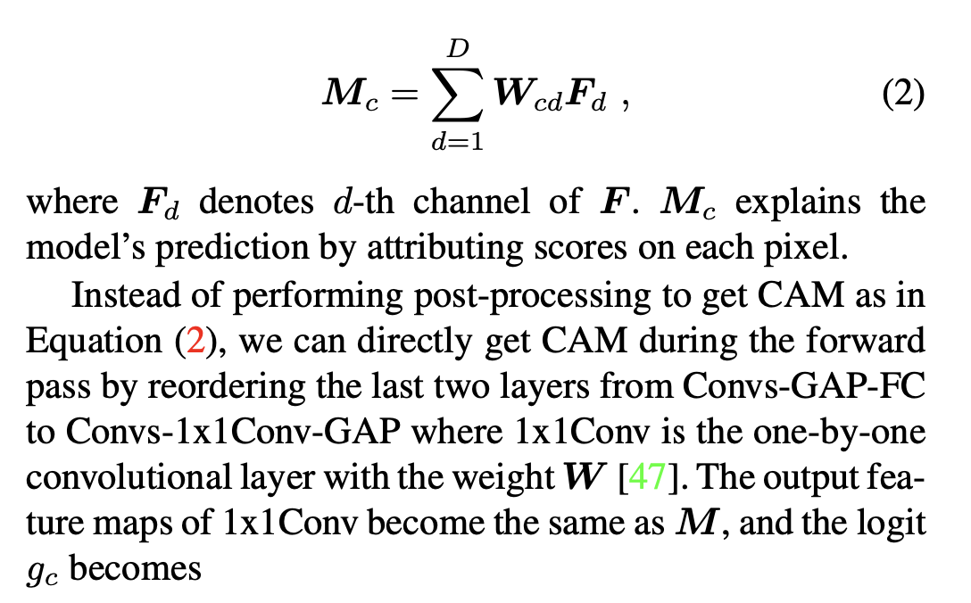
논문에서는 Recap CAM에서 모델의 구조를 수정하여 CAM을 얻는 방법을 설명하고 있다. 마지막 컨볼루션 레이어의 출력을 사용하여 CAM을 생성한다.

 

 

 

 

 

 

 

class Classifier_Module(nn.Module):
    def __init__(self, in_channels, num_classes):
        super(Classifier_Module, self).__init__()
        self.conv1x1 = nn.Conv2d(in_channels, num_classes, kernel_size=1, bias=False)
    def forward(self, x):
        cam = self.conv1x1(x)
        logits = F.adaptive_avg_pool2d(cam, (1, 1)).squeeze(-1).squeeze(-1)
        return cam, logits

 

방금 확인했던 논문 사진을 본다면 1x1 Convolution layer를 사용하여 각 클래스에 관해 CAM을 생성하는 방법을 설명하고 있다. 

we can directly get CAM during the forward pass by reordering the last two layers from Convs-GAP-FC to Convs-1x1Conv-GAP where 1x1Conv is the one-by-one convolutional layer with the weight W

 

논문에 방법에 따라GAP(Global Average Pooling)을 통해 로짓을 계산한다. 

 

 

 

 

 

def BoostLU(cam, alpha=2.0):
    boosted_cam = torch.where(cam > 0, cam * alpha, cam)
    return boosted_cam

 

논문의 main idea인 알고리즘이다. False negative이 CAM에 미치는 Impact에 대한 여러 experiment를 한 결과

 

 

 

 

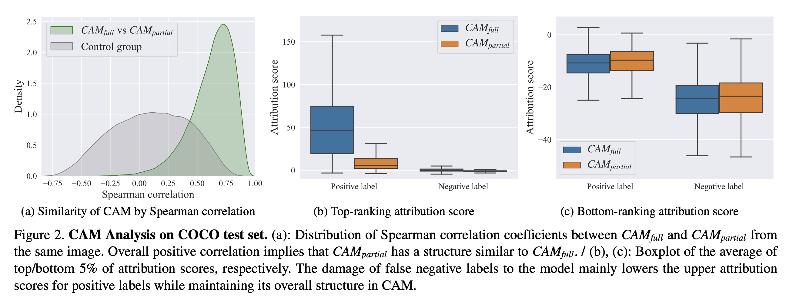
The damage of false negative labels to the model mainly lowers the upper attribution scores for positive labels while maintaining its overall structure in CAM.

 

다음 사진과 같이 Bottom-ranking attribution score 보다 Top-ranking attribution score에 대해 positive, negative label의 지표 차이가 많이 발생한 것을 볼 수 있다. 

 

 

 

 

 

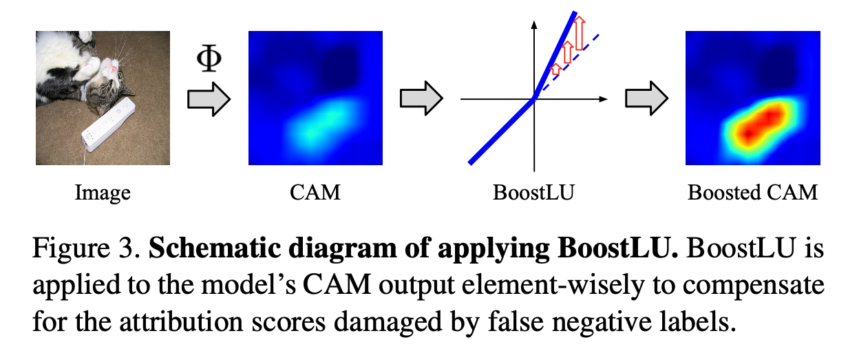
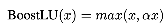
CAM의 양수인 부분에 스케일 팩터 α를 곱하여 증폭시킨다. 이 함수는 CAM의 높은 기여도를 가진 부분을 증폭하여 모델의 성능을 향상시키는 역할을 한다. 자세한 설명, 논문 코드의 전후 맥락은 여기

 

 

 

 

class MultiLabelClassifier(nn.Module):
    def __init__(self, num_classes, pretrained=True, use_boostlu=False, alpha=2.0):
        super(MultiLabelClassifier, self).__init__()
        self.backbone = ResNet101_Backbone(pretrained=pretrained)
        self.classifier = Classifier_Module(self.backbone.in_features, num_classes)
        self.use_boostlu = use_boostlu
        self.alpha = alpha
    def forward(self, x):
        features = self.backbone(x)
        cam, logits = self.classifier(features)
        if self.use_boostlu:
            cam = BoostLU(cam, alpha=self.alpha)
            logits = F.adaptive_avg_pool2d(cam, (1, 1)).squeeze(-1).squeeze(-1)
        return logits, cam

 

백본 모델과 분류기를 결합하여 멀티레이블 분류 모델을 구성한다. use_boostlu를 통해 BoostLU 함수의 사용 여부를 선택할 수 있다. 

Usage 1: BoostLU in inference only 및 Usage 2: BoostLU in both training and inference에서 BoostLU를 모델의 인퍼런스 및 훈련 단계에서 적용하는 방법을 재현하였다. 

 

 

 

 

def compute_loss(logits, labels):
    mask = labels != -1
    if mask.sum() == 0:
        return torch.tensor(0.0, requires_grad=True).to(logits.device)
    logits = logits[mask]
    labels = labels[mask].float()
    loss = F.binary_cross_entropy_with_logits(logits, labels)
    return loss

 

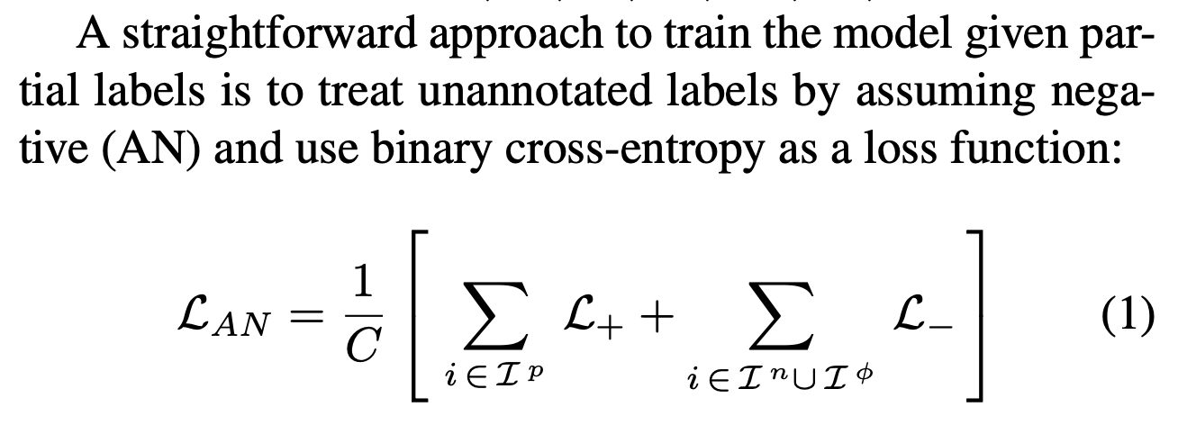
partial label (-1)을 고려하여 이진 Cross entropy Loss를 계산한다. 논문에서는 관찰되지 않은 label을 음성으로 간주하거나 무시하는 방법을 사용한다. 이것을 AN(Assume Negative) 라고 한다. 자세한 설명은 여기에

 

 

 

num_epochs = 5
for epoch in range(num_epochs):
    model.train()
    total_loss = 0
    for images, labels in train_loader:
        images = images.to(device)
        labels = labels.to(device)
        optimizer.zero_grad()
        logits, cam = model(images)
        loss = compute_loss(logits, labels)
        loss.backward()
        optimizer.step()
        total_loss += loss.item()
    avg_loss = total_loss / len(train_loader)
    print(f"Epoch [{epoch+1}/{num_epochs}], Loss: {avg_loss:.4f}")

 

이제 모델을 훈련시키기 위해 Training Loop를 구현하고, 훈련 시각화를 위해 각 Epoch 마다 손실을 출력한다. 

 

 

 

 

# 모델 평가
model.eval()
total_correct = 0
total_samples = 0
with torch.no_grad():
    for images, labels in test_loader:
        images = images.to(device)
        labels = labels.to(device)
        logits, cam = model(images)
        predictions = torch.sigmoid(logits)
        predicted_labels = (predictions > 0.5).float()
        correct = (predicted_labels == labels).float()
        correct[labels == -1] = 0
        total_correct += correct.sum().item()
        total_samples += (labels != -1).sum().item()
accuracy = total_correct / total_samples
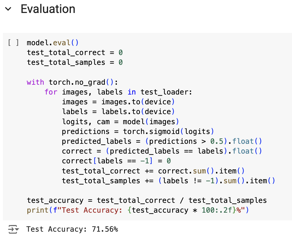
print(f"Test Accuracy: {accuracy * 100:.2f}%")

 

테스트 데이터셋에서 모델의 Accuracy를 평가하고 정확도를 출력한다. 

 

아래 사진은 Epoch 5, 한번도 수정하지 않은 Test Accuracy 수치이다.

Epoch 수를 수정하거나, 여러 hyperparameter를 잘 조율하거나, layer를 다른 방식으로 쌓아보면 더 높은 Accuracy를 기대해볼 수 있을 것 같다. 

 

 

 

 

 

추가로 다음은 CAM에 대한 감을 잡기 쉬운 시각화 코드이다.

def visualize_cam(model, image, label, alpha=0.5):
    model.eval()
    image = image.to(device).unsqueeze(0)
    label = label.to(device)

    with torch.no_grad():
        logits, cam = model(image)
        predictions = torch.sigmoid(logits)
        predicted_labels = (predictions > 0.5).float()

    # CAM 추출
    cam = cam.squeeze(0)  # [num_classes, H, W]

    # 이미지를 CPU로 이동 및 변환
    image_np = image.squeeze(0).permute(1, 2, 0).cpu().numpy()
    image_np = (image_np - image_np.min()) / (image_np.max() - image_np.min())

    # 시각화할 클래스 선택 (예: 첫 번째 클래스)
    class_idx = 0  # 원하는 클래스 인덱스로 변경 가능
    cam_class = cam[class_idx].cpu().numpy()
    cam_class = cv2.resize(cam_class, (image_np.shape[1], image_np.shape[0]))
    cam_class = (cam_class - cam_class.min()) / (cam_class.max() - cam_class.min())

    heatmap = cv2.applyColorMap(np.uint8(255 * cam_class), cv2.COLORMAP_JET)
    heatmap = np.float32(heatmap) / 255
    overlay = heatmap * alpha + image_np

    plt.figure(figsize=(10,5))
    plt.subplot(1,3,1)
    plt.imshow(image_np)
    plt.title('Original Image')
    plt.axis('off')

    plt.subplot(1,3,2)
    plt.imshow(heatmap)
    plt.title('CAM Heatmap')
    plt.axis('off')

    plt.subplot(1,3,3)
    plt.imshow(overlay)
    plt.title('Overlay')
    plt.axis('off')

    plt.show()

# 테스트 데이터셋에서 이미지 선택
dataiter = iter(test_loader)
images, labels = next(dataiter)
image = images[0]
label = labels[0]

# CAM 시각화 함수 호출
visualize_cam(model, image, label)

 

 

Output:

 

 

 

 

 

 

...오늘은 논문 code reproduction을 해보았다. 다음 번에는 팀과 같이 연구중인 것에 대해 게시물을 올릴 예정이다